Amdahl's Law and the Limits to Growth

A search service processes 350 requests per second. The server has 16 cores and the CPU utilisation is at 40%. As traffic is growing, the team believes there must be room for improvement.

They double the thread pool to 400 so that more requests can be processed simultaneously. Throughput rises from 350 to 410. With 800 threads: 425. With 1,600, it rises to 430. More threads mean almost no gain. It’s enough to make you tear your hair out!

Why is the curve flattening out? A thread dump or a look at the wall-clock profile in the profiler provides the answer: hundreds of threads are blocked. They are waiting for connections, locks and GC safe points.

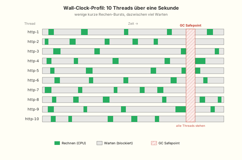
Not all processes can be fully parallelised when handling requests. Each thread requires a connection from the pool, and the database uses locks to serialise concurrent accesses at the other end. The in-memory cache synchronises via a mutex. More threads mean more object allocation and thus more frequent ‘stop-the-world’ garbage collection pauses, in which all threads are halted regardless of how many cores are available. Even modern collectors such as ZGC or Shenandoah cannot eliminate these pauses completely; they merely shorten them.

In our scenario, the search service is still a monolith that communicates with a database. In distributed systems, synchronous calls to downstream services are added – we will come to this later in the series.

All of these are serial fractions – parts of the system that every thread must pass through individually. And there is a formula that describes exactly how severely these sections limit scalability.

The upper limit

A painter is painting a flat. He spends two hours masking off the edges and sockets. He has to do this alone because each edge depends on the one before it. In theory, at least. Then he spends eight hours painting the walls. He can get help with this: two painters can do it in four hours and four in two. But the two hours of masking remain. Even with a hundred painters, the job would still take at least two hours – the serial nature of the process sets the lower limit.

Gene Amdahl formulated this in 1967. He considered a program that could be executed partly sequentially and partly in parallel and asked: ‘If I use $n$ processors, how much faster will the program run?’

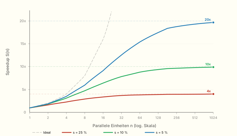
The answer can be summarised in a single sentence. The maximum speedup is the reciprocal of the serial portion. For example, if a tenth of the program is serial, the maximum speedup is a factor of ten. If a quarter of the program is serial, the maximum speedup is a factor of four. This remains true no matter how many processors are used. Formally, it looks like this:

\[S(n) = \frac{1}{s + \frac{1-s}{n}}\]

• $s$ is the proportion of the program that must be executed serially – i.e. cannot be parallelised.
• $n$ is the number of parallel units (cores, threads, instances, renderers, etc.).
• $S(n)$ is the resulting speedup.

What happens as $n$ approaches infinity? The term $\frac{1-s}{n}$ approaches zero, leaving:

\[S(\infty) = \frac{1}{s}\]

The figures are as follows:

Serial proportion $s$	Maximum speedup
50 %	2×
25 %	4×
10 %	10×
5 %	20×
1 %	100×

No matter how many cores or threads you add to a 25% serial system, it will never run more than four times faster. This is not a question of implementation, but a hard limit. If we aren’t aware of this, we’re just throwing money at cloud providers. Pointlessly.

A common pitfall here is reading $s$ from the profiler of a parallelised application instead of measuring the original execution time on a single core. If the profiler shows ‘5% serial time’ with 16 cores, this does not mean that $s = 0{,}05$ – after all, the other 95% is already distributed across the 16 cores. The actual serial proportion is significantly higher.

Amdahl’s law therefore describes an upper limit for the speedup, i.e. the best-case scenario. In practice, however, things often turn out worse because the coordination overhead between parallel units can actively reduce throughput, not just cause it to stagnate. The team working on the search service was fortunate in that the throughput merely stagnated. In other systems, such as when many threads compete for the same database rows or retry storms flood the network, throughput can plummet dramatically.

Originally, the law describes the acceleration of a fixed workload. However, the same mechanism also applies when many requests per second pass through a system. Each request is a fixed job that must pass through the same serialisation point, which is why Amdahl’s law applies to both the latency of the individual request and, via Little’s law, to the overall throughput. Little’s law links parallelism, throughput and response time. This is precisely what the search service experienced at 430 req/s, even though there was still free capacity on the cores.

Digression: The Universal Scalability Law – Amdahl is a hopeless optimist

„The purpose of models is not to fit the data but to sharpen the questions.” – Sam Karlin, quoted by Neil Gunther

In 1993, Neil Gunther enhanced Amdahl’s model by a second term and developed the Universal Scalability Law (USL). Alongside the serial component $\sigma$ (contention, which corresponds to Amdahl’s $s$), Gunther introduced a coherence parameter $\kappa$ (crosstalk).

\[C(n) = \frac{n}{1 + \sigma(n-1) + \kappa \times n \times (n-1)}\]

The key difference lies in the last term: $\kappa \times n \times (n-1)$ grows quadratically with the number of units. If $\kappa = 0$ (no coordination overhead), the formula reduces to Amdahl’s Law. As soon as $\kappa > 0$, there is a point beyond which the coordination overhead exceeds the gains from parallelisation. The throughput decreases.

Imagine an overzealous department manager who gets involved in every detail. According to Amdahl’s Law, no matter how many employees are in the department, the manager remains the bottleneck – adding more people doesn’t help at a certain point. Gunther adds that employees also have to coordinate with each other to decide who goes to the manager with which issue. At a certain team size, they spend more time coordinating than working.

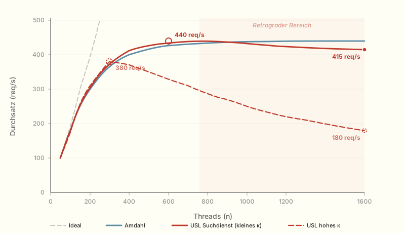
In the search service, the impact is minimal: cache line bouncing, context switching and the occasional lock convoy account for a few per cent. At 1,600 threads, throughput reaches a maximum of 435 req/s, dropping to 415 instead of the predicted 430 based on a pure Amdahl’s law calculation. This is annoying, but not a major issue. This is because the threads spend most of their time waiting for I/O and rarely interfere with each other. The $\kappa$ of the search service is small.

In systems that require a great deal of coordination, however, the situation is different. For example, a database server that spends more time on lock management than on queries as the number of connections increases. A message broker that spends more time on rebalancing than on delivery as the number of consumers grows. Distributed caches in which every write operation must be propagated to all nodes. In such systems, the throughput drops significantly – not by a few per cent, but to a fraction of the maximum.

The solid red line shows the search service, which experiences a slight decline that primarily incurs costs. The dotted red line shows what happens with strong coordination: the retrograde region, where each additional unit actively degrades the system. Amdahl’s law is the most optimistic of the scaling laws. The USL shows just how far reality can deviate from it.

Gunther summarises the three barriers to scaling as the ‘3 Cs’: Concurrency (ideal parallelism), Contention ($\sigma$, waiting time for shared resources) and Coherence ($\kappa$, the effort required to establish a consistent state between parallel units). This is a useful diagnostic framework: if a system fails to scale, the reason is either insufficient parallelism, resource contention, or coordination overhead. Contention $\sigma$ and coherency $\kappa$ can be determined empirically from load test data, meaning that coupling shifts from a design principle to a measurable system property.

What does ‘serial’ mean?

Amdahl was thinking of parallel computers: multiple processors, a single program. But the model is more general. Wherever parallel units encounter shared resources, the same principle applies. The serial component is every shared resource and every central coordination point:

• A mutex that protects a shared data structure is a serialising element. Multiple threads compete for the same lock; throughput does not scale with the number of threads.
• A database that all requests write to is a serial component. Increasing the thread pool and connection pool makes no difference – the bottleneck lies at the other end of the connection, just as observed in the introduction.
• A synchronous HTTP or gRPC call to another service is a serial operation. The thread waits for the response in a blocking manner, regardless of how many cores are available locally. Virtual threads (Java 21) mitigate this local issue – the thread waits without blocking the pool – but the serial nature remains: The downstream service can only process a limited number of requests per unit of time. This bottleneck grows linearly with the number of downstream dependencies: anyone who breaks down a monolith into five synchronously coupled services has quintupled the serial bottleneck per request, rather than reducing it – and at the same time has worsened availability and response times.
• Even seemingly harmless (standard) libraries can conceal serialised components. Java’s Math.random() uses a shared seed internally: each call competes for the same value in a loop – the loser tries again until it gets a turn. System.out.println() maintains a global monitor. In .NET, Random wasn’t even thread-safe prior to version 6. The solution is always the same: thread-local alternatives such as ThreadLocalRandom or Random.Shared. But the shared default is often the trap you fall into first. You can’t tell by looking at the libraries – only a profiler can help. A tool that, for reasons beyond my comprehension, is hardly used anymore these days.

But what exactly happens at the p99 when these serial sections come under load?

Tail Latency

In addition to capping the maximum throughput, the serial component has another effect: it increases the response time at the tail end of the distribution. This is precisely where the SLAs come into play.

The explanation comes from Kingman’s formula – the interplay between utilisation and variability: Queues do not grow uniformly when utilisation is high, but rather in an explosive manner. The effect is represented by the term $\frac{\rho}{1 - \rho}$, where $\rho$ is the utilisation of the serial section. At 80% utilisation, this term has a value of 4; at 90%, it is already 9; at 95%, it is 19. When utilisation rises from 80% to 90%, the average waiting time roughly doubles, whilst the p99 value quadruples.

The more threads that compete for the same lock, the more likely it is that a single request will end up at the back of a long queue – and this is precisely the request that will appear in the p99. This is yet another reason why monitoring should not focus solely on the mean, but rather on the distribution of response times.

This issue is exacerbated in service landscapes. A request that calls on five downstream services, either in parallel or sequentially, is highly likely to encounter at least one of them at an inopportune moment. With every additional synchronous hop, the probability of getting stuck in at least one of the queues increases. In formal terms, with $N$ services, each of which responds slowly in 1% of cases, the probability of encountering at least one slow response is $1 - 0{,}99^N$ – just under 5% for five services and almost 10% for ten.

The p99 of the overall response is therefore dominated by the p99 of the individual services rather than the mean. Delimitrou and Kozyrakis formalised this in 2018 as Amdahl’s Law for Tail Latency: the serial component determines not only whether throughput increases, but also how predictably the system responds under load.

In the case of tail latency, both laws apply: increased parallelism reaches the Amdahl limit whilst rising utilisation causes waiting times to grow disproportionately in accordance with Kingman’s law.

This can also be put to practical use. If the spread between P50 and P99 widens as the load increases, this provides empirical evidence that serial sections are experiencing contention. In purely parallel processing, response times would be consistent: some requests would be fast, while others of the same type would be ten times slower. Some requests would arrive at an empty queue, while others would have to wait. A growing P99/P50 ratio indicates that serialisation is becoming problematic, even before you fire up the profiler.

From a thread to a team

All of this applies to a single instance, but the same effect is repeated at every level. Within an instance, threads share caches, connection pools, and lock-protected data structures. One level down, the database is parallelised across cores but serialises write operations via locks; ACID enforces this. As soon as multiple instances of the same service access the same database, the serialised portion simply moves one level down, a topic we will explore in more detail in the next two parts.

This principle does not stop at technology, either. Just as locks slow down threads, shared codebases and centralised decision-makers slow down teams. Theoretical principles of scalability apply to all forms of parallelism, including hardware, software and organisational structures.

The result is always the same: Loose coupling – minimal shared resources, maximum autonomy. The extreme variant, Shared-Nothing, eliminates shared resources entirely, meaning there is no shared memory, database or locks. In practice, this is a rare ideal that is rarely fully achieved. However, every step in that direction pushes the Amdahl limit upwards because the amount of serial components is reduced.

Architecture beats hardware

Let’s go back to the search service. The team is aware of the serialisation points — the connection pool, the cache mutex and the DB locks — but how significant is the serialised portion in reality? To find out, they deployed the service on various instance sizes within the AWS c7g family and ran the same load test on each one until it reached saturation.

Instance type	vCPUs	Throughput (saturation)	Speedup vs. 2 cores	Price per hour
c7g.large	2	175 req/s	1,0×	1×
c7g.xlarge	4	260 req/s	1,5×	2×
c7g.2xlarge	8	345 req/s	2,0×	4×
c7g.4xlarge	16	430 req/s	2,5×	8×

The pattern is clear: each doubling of the number of cores yields less than the previous one. The team fits the Amdahl curve to the measurement data and arrives at $s \approx 0.20$ – around one-fifth of the processing time is spent in serial processing. This means that the theoretical upper limit for the speedup is five, regardless of how many cores are used. On the current 16 cores, the formula gives $S(16) = \frac{1}{0.20 + 0.80/16} = 4.0\times$ – which matches the measured 430 req/s.

The obvious question is: what would happen if you simply bought a more powerful machine? As the table shows, every doubling of the number of cores doubles the price, but the throughput increases at an ever-slower rate. For example, upgrading from 16 to 32 vCPUs would provide an additional 11% performance increase at 100% extra cost. With 64 cores, you get another 7% on top of that. You’d have to be keen on that. At some point, however, the options run out: at 64 vCPUs with AWS and at 176 with GCP. After that, there simply aren’t any larger machines available.

The more worthwhile investment: reducing the serial portion. Better indices, asynchronous processing, lock-free data structures – reducing $s$ from 20% to 10% doubles the speedup ceiling from five to ten. On the same 16 cores, the theoretical speedup rises from 4.0× to 6.4×. Architecture trumps hardware.

For the search service, this indicates that the instance has reached its limit. Adding more cores makes little difference, and adding more threads makes no difference at all. The most obvious next step would be to simply run more instances alongside it. However, the serial part doesn’t disappear; it just shifts elsewhere.

---

Sources

• Amdahl (1967) – Validity of the single processor approach to achieving large scale computing capabilities. AFIPS Spring Joint Computer Conference Proceedings, Vol. 30, 483–485.
• Gustafson (1988) – Reevaluating Amdahl’s Law. Communications of the ACM, 31(5), 532–533.
• Gunther (1993) – Practical Performance Analyst. McGraw-Hill. → Universal Scalability Law
• Gunther (2007) – Guerrilla Capacity Planning. Springer. → USL formalised and applied
• Delimitrou & Kozyrakis (2018) – Amdahl’s Law for Tail Latency. Communications of the ACM, 61(8), 65–72.
• Abbott & Fisher (2015a) – The Art of Scalability. 2nd ed., Chapter 22. Addison-Wesley.

Comments